|
|

|
|
|
|
This page presents the basic usages of ULySS to fit a spectrum against
stellar templates, with a model of atmosphere or with stellar population
models.
The tutorials are written to follow a smooth progression, from commands
requiring minimal understanding of the method (ulyss, <my_spectrum>), to examples demonstrating the flexibility of the package
(make composite fits, set constraints on the parameters...).
GDL> star = uly_root+'/data/cflib_114642.fits'
GDL> ulyss, star
Use default model: Solar spectrum
--------------------------------------------------------------------
INPUT PARAMETERS
--------------------------------------------------------------------
The fits file to be analyze is       ./data/cflib_114642.fits
Name of the output file              output.res
Degree of multiplicative polynomial            10
No additive polynomial
Component1 (cmp1) file:./models/sun.fits
--------------------------------------------------------------------
--------------------------------------------------------------------
PARAMETERS PASSED TO ULY_FIT
--------------------------------------------------------------------
Wavelength range used                 :       3464.9160       9469.5171
 [Angstrom]
Sampling in log wavelength            :       20.079155 [km/s]
Number of independent pixels in signal:       15011
Number of pixels fitted               :       15011
DOF factor                            :      1.00000
--------------------------------------------------------------------
number of model evaluations:          35
time=       1.5249200
Number of pixels used for the fit       15007

cz             :       7.5581444 +/- 0.96103474 km/s
dispersion     :       75.070373 +/- 0.88710896 km/s
-----------------------------------------------
estimated SNR  :       12.510639
-----------------------------------------------
cmp #0  cmp1
Weight         :    0.0057345585 +/-    5.3433868e-05 [data_unit/cmp_unit]
-----------------------------------------------
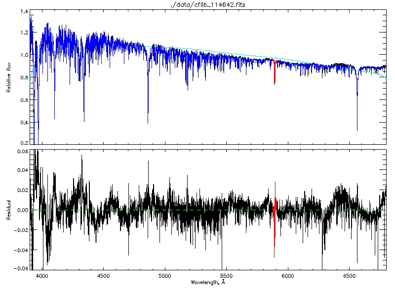
GDL> ulyss, star, MODEL_FILE=uly_root+'/models/elodie32_flux_tgm.fits', /PLOT
--------------------------------------------------------------------
INPUT PARAMETERS
--------------------------------------------------------------------
The fits file to be analyze is       ./data/cflib_114642.fits
Name of the output file              output.res
Degree of multiplicative polynomial            10
No additive polynomial
Component1 (cmp1) model:./models/elodie32_flux_tgm.fits
  Guess for Teff: 7000.0000 [K], Logg: 2.0000000 [cm/s2], Fe/H: 0.0000000 [dex]
--------------------------------------------------------------------
--------------------------------------------------------------------
PARAMETERS PASSED TO ULY_FIT
--------------------------------------------------------------------
Wavelength range used                 :       3900.2338       6800.1479
 [Angstrom]
Sampling in log wavelength            :       20.079155 [km/s]
Number of independent pixels in signal:        8300
Number of pixels fitted               :        8300
DOF factor                            :      1.00000
--------------------------------------------------------------------
number of model evaluations:          68
time=       2.7778258
Number of pixels used for the fit        8218

cz             :       1.3043659 +/- 0.14290816 km/s
dispersion     :       31.781528 +/- 0.15732457 km/s
-----------------------------------------------
estimated SNR  :       77.287751
-----------------------------------------------
cmp #0  cmp1
Weight         :      0.99005952 +/-      0.010510920 [data_unit/cmp_unit]
Teff           :       6397.5471 +/- 4.0069625 K
Logg           :       4.0506557 +/- 0.0080833872 cm/s2
Fe/H           :     -0.15417556 +/- 0.0049592401 dex
-----------------------------------------------
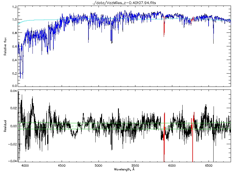
GDL> galaxy = uly_root+'/data/VazMiles_z-0.40t07.94.fits'
GDL> ulyss, galaxy, MODEL_FILE= uly_root+'/models/PHR_Elodie31.fits'
--------------------------------------------------------------------
INPUT PARAMETERS
--------------------------------------------------------------------
The fits file to be analyze is       ./data/VazMiles_z-0.40t07.94.fits
Name of the output file              output.res
Degree of multiplicative polynomial            10
No additive polynomial
Component1 (cmp1) model:./models/PHR_Elodie31.fits
  Guess for age: 8000.0000 [Myr], Fe/H: -0.40000000 [dex]
--------------------------------------------------------------------
Read the model ./models/PHR_Elodie31.fits
read the file ./models/PHR_Elodie31.fits
model reading time=       1.7968800
model deriving time=      0.21679497
--------------------------------------------------------------------
PARAMETERS PASSED TO ULY_FIT
--------------------------------------------------------------------
Wavelength range used                 :       3900.5447       6800.7178
 [Angstrom]
Sampling in log wavelength            :       51.501300 [km/s]
Number of independent pixels in signal:        3236
Number of pixels fitted               :        3236
DOF factor                            :      1.00000
--------------------------------------------------------------------
number of model evaluations:          52
time=      0.51620889
Number of pixels used for the fit        3172

cz             :       6.4171465 +/- 0.29640537 km/s
dispersion     :       62.357711 +/- 0.30356847 km/s
-----------------------------------------------
estimated SNR  :       107.19732
-----------------------------------------------
cmp #0  cmp1
Weight         :       1.0981672 +/-    6.8035115e-05 [data_unit/cmp_unit]
age            :       6355.5287 +/- 109.68133 Myr
Fe/H           :     -0.36017315 +/- 0.0065616429 dex
-----------------------------------------------
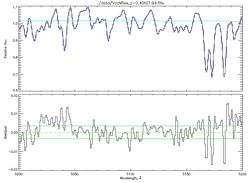
GDL> galaxy = uly_root+'/data/VazMiles_z-0.40t07.94.fits'
GDL> spectrum = uly_spect_read(galaxy)
GDL> specConv = uly_spect_losvdconvol(spectrum, 0., 30., 0, 0)
GDL> uly_spect_free, spectrum
GDL> ulyss, specConv, MODEL='models/PHR_Elodie31.fits', /QUIET, FILE_OUT='tuto_base'
GDL> uly_solut_tprint, 'tuto_base.res'
GDL> uly_solut_splot, 'tuto_base.fits', WAVERANGE=[5000.,5200.]
cz             :       6.3734618 +/- 0.37938520 km/s
dispersion     :       68.989962 +/- 0.38664303 km/s
-----------------------------------------------
estimated SNR  :      113.996
-----------------------------------------------
cmp #0  cmp4
Weight         :       1.1169801 +/-    6.9208513e-05 [data_unit/cmp_unit]
age            :       6497.0194 +/- 130.65446 Myr
Fe/H           :     -0.36589060 +/- 0.0074055300 dex
-----------------------------------------------
GDL> galaxy = uly_root+'/data/VazMiles_z-0.40t07.94.fits'
GDL> cmp1 = uly_ssp(AG=[1000.], ZG=[0], AL=[200.,3000.])
GDL> cmp2 = uly_ssp(AG=[10000.], ZG=[0], AL=[3000., 12000.])
GDL> cmp = [cmp1, cmp2]
GDL> ulyss, galaxy, cmp, /PLOT
--------------------------------------------------------------------
INPUT PARAMETERS
--------------------------------------------------------------------
The fits file to be analyze is       ./data/VazMiles_z-0.40t07.94.fits
Name of the output file              output.res
Degree of multiplicative polynomial            10
No additive polynomial
Component1 (cmp1) model:./models/PHR_Elodie31.fits
  Guess for age: 1000.0000 [Myr], Fe/H: 0.0000000 [dex]
Component2 (cmp2) model:./models/PHR_Elodie31.fits
  Guess for age: 10000.000 [Myr], Fe/H: 0.0000000 [dex]
--------------------------------------------------------------------
Read the model ./models/PHR_Elodie31.fits
read the file ./models/PHR_Elodie31.fits
model reading time=       1.7573318
model deriving time=      0.21527600
Read the model ./models/PHR_Elodie31.fits
read the file ./models/PHR_Elodie31.fits
model reading time=       1.7630351
model deriving time=      0.21560097
--------------------------------------------------------------------
PARAMETERS PASSED TO ULY_FIT
--------------------------------------------------------------------
Wavelength range used                 :       3900.5447       6800.7178
 [Angstrom]
Sampling in log wavelength            :       51.501300 [km/s]
Number of independent pixels in signal:        3236
Number of pixels fitted               :        3236
DOF factor                            :      1.00000
--------------------------------------------------------------------
number of model evaluations:          45
time=      0.73431396
Number of pixels used for the fit        3172

cz             :       6.4343579 +/- 0.30888007 km/s
dispersion     :       62.408533 +/- 0.31547613 km/s
-----------------------------------------------
estimated SNR  :       104.62244
-----------------------------------------------
cmp #0  cmp1
Light fraction :       3.3730552 +/-      0.066524257 %
Weight         :     0.014335284 +/-    0.00028272413 [data_unit/cmp_unit]
age            :       2374.2576 +/- 77896.473 Myr
Fe/H           :     -0.52676316 +/- 31.854347 dex
-----------------------------------------------
cmp #1  cmp2
Light fraction :       96.626945 +/-      0.066056484 %
Weight         :       1.0035757 +/-    0.00068606830 [data_unit/cmp_unit]
age            :       5940.4404 +/- 206.11379 Myr
Fe/H           :     -0.36143326 +/- 0.0083828031 dex
-----------------------------------------------
GDL> star = uly_root+'/data/cflib_114642.fits'
GDL> model = uly_tgm_extr(star,[6400.,4.,0.]) ;  Teff=6400K log(g)=4 [Fe/H]=0
GDL> cmp = uly_star(model)
GDL> uly_lsf, star, cmp, 600, 300, FILE='tuto_lsf.txt', /QUIET
GDL> plotsym,0,1,/FILL
GDL> uly_lsf_plot, 'tuto_lsf.txt', YST=3, PSYM=8, CONNECT='Red'
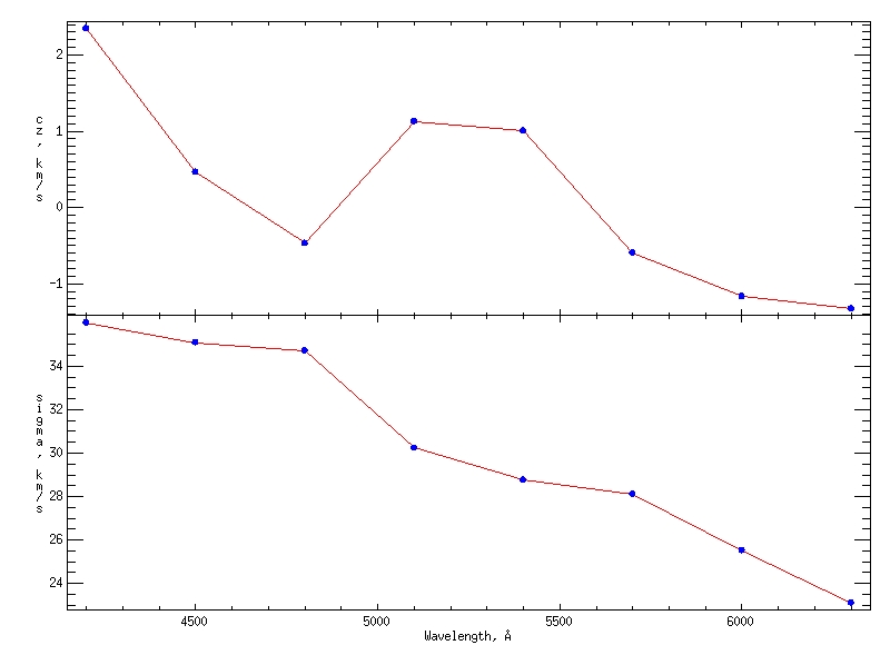
GDL> uly_lsf_smooth, 'tuto_lsf.txt', 'tuto_lsf_s.txt'
GDL> galaxy = uly_root+'/data/VazMiles_z-0.40t07.94.fits'
GDL> cmp = uly_ssp(LSF='tuto_lsf_s.txt')
GDL> ulyss, galaxy, cmp, /QUIET
| Contact: ulyss at obs.univ-lyon1.fr |
Last modified: Thu Jul 31 13:57:09 2008. |