|
|

|
|
|
|
GDL> ; power is the component structure describing the power-low component
GDL> power = {name:'power', $
GDL>          descr:'Power-law component -- demonstration', $
GDL>          init_fun:'', $
GDL>          init_data:ptr_new(), $
GDL>          eval_fun:'tuto_power', $
GDL>          eval_data:ptr_new(/ALLO), $ ; will be filled by ULY_FIT_INIT
GDL>          para:ptr_new(/ALLO), $
GDL>          start:0d, $              ; this will be filled by ULY_FIT_INIT
GDL>          step:0d, $               ; this will be filled by ULY_FIT_INIT
GDL>          npix: 0l, $              ; this will be filled by ULY_FIT_INIT
GDL>          sampling:-1s, $          ; this will be filled by ULY_FIT_INIT
GDL>          mask:ptr_new(), $
GDL>          weight:0d, $
GDL>          e_weight:0d, $
GDL>          l_weight:0d, $
GDL>          lim_weig:[!VALUES.D_NaN,!VALUES.D_NaN] $
GDL>         }
GDL>
GDL> ; We have also to define the para structure, describing the parameter tau:
GDL> *power.para = {name:'tau', unit:'', guess:ptr_new(0D), step:1D-2, $
GDL>                        limits:[-10d,10d], limited:[1,1], fixed:0S, $
GDL>                        value:0D, error:0D, dispf:''}
GDL>
GDL> ; Since init_func is empty, ULY_FIT_INIT will fill the WCS information
GDL> ; with the values corresponding to the spectrum to fit, and will
GDL> ; pass the cmp structure as eval_data.
function tuto_power, eval_data, pars
; pars is the array of parameters, actually only one value: the exponent
step = eval_data.step
npix = eval_data.npix

; simply return the array:
return, exp(findgen(npix)*step*pars[0])

end
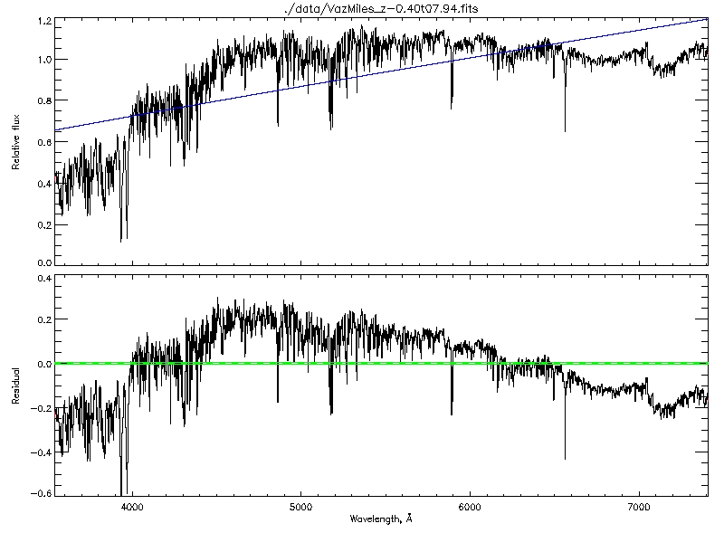
GDL> ; Choose a galaxy spectrum to test this model, and try the fit
GDL> galaxy = uly_root+'/data/VazMiles_z-0.40t07.94.fits'
GDL> ulyss, galaxy, power, KMOMENT=0, MD=0, /PLOT
--------------------------------------------------------------------
INPUT PARAMETERS
--------------------------------------------------------------------
The fits file to be analyze is       ./data/VazMiles_z-0.40t07.94.fits
Name of the output file              output.res
Degree of multiplicative polynomial         0
No additive polynomial
Component1 (power) Power-law component -- demonstration
  Guess for tau: 0.0000000 []
--------------------------------------------------------------------
--------------------------------------------------------------------
PARAMETERS PASSED TO ULY_FIT
--------------------------------------------------------------------
Wavelength range used                 :       3540.3541       7410.6865
 [Angstrom]
Sampling in log wavelength            :       51.501300 [km/s]
Number of independent pixels in signal:        4300
Number of pixels fitted               :        4300
DOF factor                            :      1.00000
--------------------------------------------------------------------
number of model evaluations:          20
time=      0.26058793
Number of pixels used for the fit        4296
-----------------------------------------------
estimated SNR  :       5.5137068
-----------------------------------------------
cmp #0  power
Weight         :       193.34682 +/-      0.010987264 [data_unit/cmp_unit]
tau            :      0.80914968 +/- 0.013234491
-----------------------------------------------
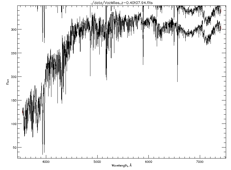
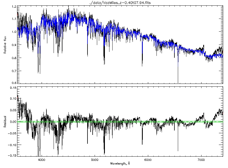
GDL> g = uly_spect_read(uly_root+'/data/VazMiles_z-0.40t07.94.fits')
GDL> g = uly_spect_logrebin(g, /OVERWRITE)
GDL> tau = -3d
GDL> p = exp(findgen(n_elements(*g.data))*g.step*tau)
GDL> *g.data += 0.5 * mean(*g.data)/mean(p) * p
GDL>
GDL> window, 0
GDL> uly_spect_plot, galaxy, LINECOLOR='Black'
GDL> uly_spect_plot, g, /OVERPLOT
GDL>
GDL> window, 1
GDL> cmp = [power, uly_ssp(MODEL_FILE=uly_root+'/models/Vaz_Miles.fits')]
GDL> ulyss, g, cmp, KMOMENT=0, MD=0, /PLOT
--------------------------------------------------------------------
INPUT PARAMETERS
--------------------------------------------------------------------
Name of the output file              output.res
Degree of multiplicative polynomial         0
No additive polynomial
Component1 (power) Power-law component -- demonstration
  Guess for tau: 0.0000000 []
Component2 (cmp1) model:./models/Vaz_Miles.fits
  Guess for age: 8000.0000 [Myr], Fe/H: -0.40000000 [dex]
--------------------------------------------------------------------
Read the model ./models/Vaz_Miles.fits
read the file ./models/Vaz_Miles.fits
model reading time=      0.72519398
model deriving time=      0.16913700
--------------------------------------------------------------------
PARAMETERS PASSED TO ULY_FIT
--------------------------------------------------------------------
Wavelength range used                 :       3540.3541       7410.6865
 [Angstrom]
Sampling in log wavelength            :       51.501300 [km/s]
Number of independent pixels in signal:        4300
Number of pixels fitted               :        4300
DOF factor                            :      1.00000
--------------------------------------------------------------------
number of model evaluations:          18
time=      0.25502086
Number of pixels used for the fit        4296
-----------------------------------------------
estimated SNR  :       31.287810
-----------------------------------------------
cmp #0  power
Light fraction :       64.326810 +/-      0.010470703 %
Weight         :       342.38408 +/-      0.055731070 [data_unit/cmp_unit]
tau            :     -0.84375152 +/- 0.018304158
-----------------------------------------------
cmp #1  cmp1
Light fraction :       35.673190 +/-      0.010348450 %
Weight         :      0.19057977 +/-    5.5285362e-05 [data_unit/cmp_unit]
age            :       1710.1191 +/- 37.994848 Myr
Fe/H           :      0.22000000 +/- 0.013664700 dex
-----------------------------------------------
| Contact: ulyss at obs.univ-lyon1.fr |
Last modified: Thu Jul 31 13:57:09 2008. |