|
|

|
|
|
|
One of the strength of ULySS is the set of tools included to help to
study the parameters space. The problems handled with ULySS are non-linear
and often complex enough to present degeneracies, multiple minima and
restrictions on the convergence to the absolute minimum.
This page presents some examples of Monte-Carlo simulations, chi2 maps
and convergence maps.
To follow this tutorial it is advisable first to read the general tutorial.
GDL> grid=uly_ssp_read(uly_root+'/models/PHR_Elodie31.fits', SIGMA=50., VELSCALE=50.)
GDL> young = uly_ssp_interp(grid, [alog(500.), 0.])
GDL> old = uly_ssp_interp(grid, [alog(10000.), -1.])
GDL>
GDL> spectrum = uly_spect_alloc(DATA=0.1*young+0.9*old, START=grid.start, STEP=grid.step, SAMPLING=1)
GDL> cmp1 = uly_ssp(AG=[500.], ZG=[0], AL=[200.,3000.])
GDL> cmp2 = uly_ssp(AG=[10000.], ZG=[-1.], AL=[3000., 12000.])
GDL> cmp = [cmp1, cmp2]
GDL> ulyss, spectrum, cmp
Read the model ./models/PHR_Elodie31.fits
read the file ./models/PHR_Elodie31.fits
model reading time=       1.7927818
Convolve the model with Gaussian, sigma=      50.0000 km/s
model deriving time=      0.22342515
--------------------------------------------------------------------
INPUT PARAMETERS
--------------------------------------------------------------------
Name of the output file              output.res
Degree of multiplicative polynomial            10
No additive polynomial
Component1 (cmp1) model:./models/PHR_Elodie31.fits
  Guess for age: 500.00000 [Myr], Fe/H: 0.0000000 [dex]
Component2 (cmp2) model:./models/PHR_Elodie31.fits
  Guess for age: 10000.000 [Myr], Fe/H: -1.0000000 [dex]
--------------------------------------------------------------------
Read the model ./models/PHR_Elodie31.fits
read the file ./models/PHR_Elodie31.fits
model reading time=       1.7861340
model deriving time=      0.22379780
Read the model ./models/PHR_Elodie31.fits
read the file ./models/PHR_Elodie31.fits
model reading time=       1.7899010
model deriving time=      0.22375083
--------------------------------------------------------------------
PARAMETERS PASSED TO ULY_FIT
--------------------------------------------------------------------
Wavelength range used                 :       3900.2252       6801.1087
 [Angstrom]
Sampling in log wavelength            :       50.000000 [km/s]
Number of independent pixels in signal:        3334
Number of pixels fitted               :        3334
DOF factor                            :      1.00000
--------------------------------------------------------------------
number of model evaluations:          12
time=      0.20227480
Number of pixels used for the fit        3269

cz             :       0.0000000 +/- 0.00062760970 km/s
dispersion     :       50.000000 +/- 0.00068582551 km/s
-----------------------------------------------
estimated SNR  :       54810.876
-----------------------------------------------
cmp #0  cmp1
Light fraction :       48.695512 +/-      0.014961593 %
Weight         :     0.099943584 +/-    3.0707454e-05 [data_unit/cmp_unit]
age            :       500.00000 +/- 0.022189165 Myr
Fe/H           :       0.0000000 +/- 3.9526592e-05 dex
-----------------------------------------------
cmp #1  cmp2
Light fraction :       51.304488 +/-      0.015264779 %
Weight         :      0.90047556 +/-    0.00026792121 [data_unit/cmp_unit]
age            :       10000.000 +/- 1.7618713 Myr
Fe/H           :      -1.0000000 +/- 4.6371446e-05 dex
-----------------------------------------------
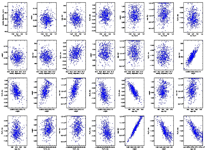
GDL> ulyss, spectrum, cmp, NSIMUL=500, SNR=100, FILE_OUT='tuto_chi', /QUIET, /PLOT
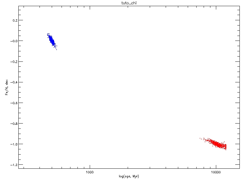
GDL> uly_solut_tplot, 'tuto_chi', XAXIS=4, YAXIS=5, XRANGE=[300.,14000.], YRANGE=[-1.2, 0.3], /XLOG
GDL> uly_solut_tplot, 'tuto_chi', XAXIS=7, YAXIS=8, /OVER, LINECOLOR='red'
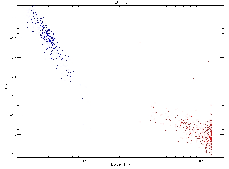
GDL> ulyss, spectrum, cmp, NSIMUL=500, FILE_OUT='tuto_chi', SNR=15, /QUIET
GDL> uly_solut_tplot, 'tuto_chi', XAXIS=4, YAXIS=5, XRANGE=[300.,14000.], YRANGE=[-1.2, 0.3], /XLOG
GDL> uly_solut_tplot, 'tuto_chi', XAXIS=7, YAXIS=8, /OVER, LINECOLOR='red'
GDL> chi1 = uly_chimap(spectrum, cmp, [[0,0],[0,1]])
GDL> chi2 = uly_chimap(spectrum, cmp, [[1,0],[1,1]])
GDL> window, 0
GDL> uly_chimap_plot, chi1, /XLOG, YRANGE=[-1.2, 0.3]
GDL> window, 1
GDL> uly_chimap_plot, chi2, /XLOG, YRANGE=[-1.2, 0.3]
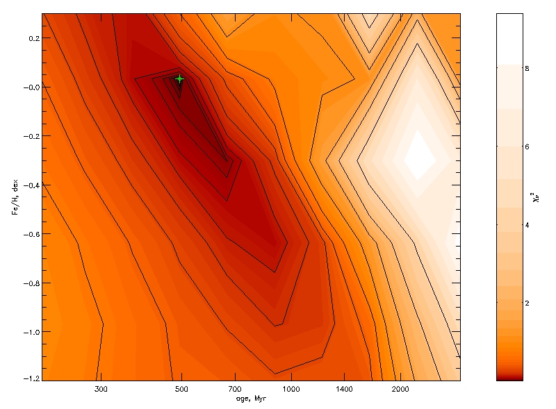
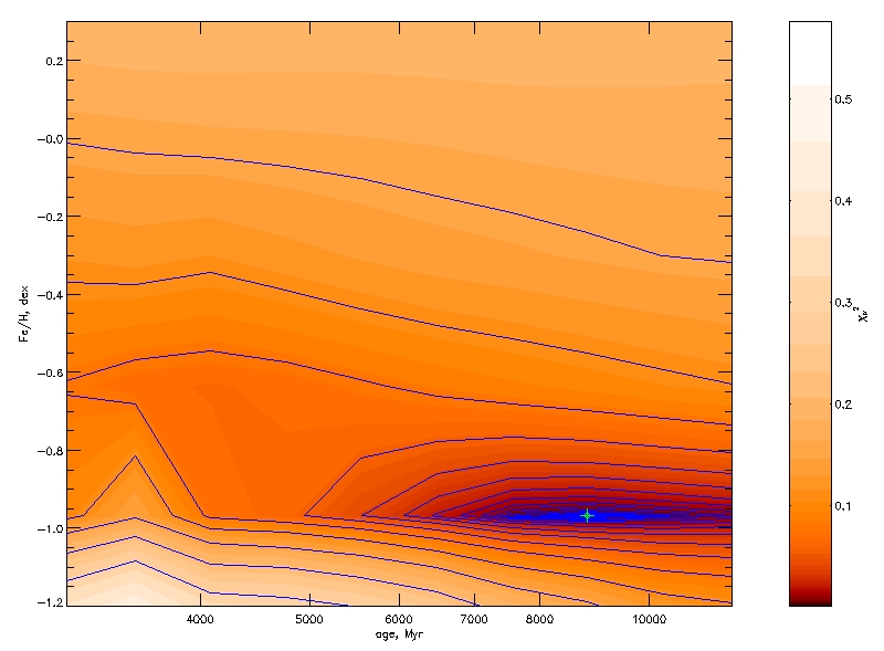
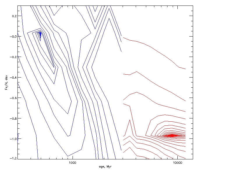
GDL> uly_chimap_plot, chi1, XRANGE=[300.,14000.], /XLOG, YRANGE=[-1.2, 0.3], /HIDEHALFTONE, /HIDEMINIMA
GDL> uly_chimap_plot, chi2, /HIDEHALFTONE, /HIDEMINIMA, /OVER, LINECOLOR='red'
GDL> gal=uly_root+'/data/VazMiles_z-0.40t07.94.fits'
GDL> cmp = uly_ssp(AG=[500d,1000d,2000d,4000d,8000d,15000d,18000d], ZG=[-2d,-1.5d,-1d,-0.5d,0d,0.3d])
GDL> ulyss, gal, cmp, /ALL_SOL, FIL='absolute'
GDL> uly_solut_tplot, 'absolute.res', XA=[0,0], YA=[0,1], XR=[300,25000], YR=[-1.6,0.5], /CV, /XLOG

| Contact: ulyss at obs.univ-lyon1.fr |
Last modified: Thu Jul 31 13:57:09 2008. |