Home Download Tutorial 1 Tutorial 2 Tutorial 3 Tutorial 4 Tutorial 5

ULySS includes a variety of plotting subroutines geared towards displaying all usefull information about the fits and their results.
This tutorial presents some of these plotting tasks and the general plotting philosophy of ULySS.

To follow this tutorial it is advisable first to read the general tutorial.

1. General considerations

For many high level task, you can use the /PLOT keyword to imediatly see the result. This is the case for the ulyss main task (as well as several others):
GDL> star = uly_root+'/data/cflib_114642.fits'
GDL> ulyss, star, /plot, /quiet
For practical reasons, these high level tasks plotting capacities are quite basic and have only been included for conveniency. All plot parameters are set to default and are essentially non-customizable. Of course, this may or may not suit your specific needs and you might wish to change some of the plotting details. For this, you will have to se the specific plotting tasks that are included in the ULySS package. The above plot, for example, can be reproduced with the following commands:
GDL> star = uly_root+'/data/cflib_114642.fits'
GDL> ulyss, star, SOLUTION=solution, /quiet
GDL> uly_solut_splot, solution

2. Basic plot customization

Every plotting tasks use a structure containing all the plot variables such as colors, line styles, etc. This structure can be obtained by running the following command:
GDL> plot_var = uly_plot_init()
This initializing task is automatically called by the plotting subroutine if the structure is not supplied. So, the following commands are strictly equivalent:
GDL> uly_solut_splot, solution
and
GDL> plot_var = uly_plot_init()
GDL> uly_solut_splot, solution, PLOT_VAR=plot_var
but the latter allows for customization. There are two ways to change the plotting behaviour. The first is to initialise plot_var with the desired settings, the second is to modify the plot_var structure.
GDL> window, 0
GDL> plot_var = uly_plot_init(POLYCOLOR='Grey', POLYSTYLE=2)
GDL> uly_solut_splot, solution, TITLE='Example1', PLOT_VAR=plot_var
GDL> window, 1
GDL> plot_var.polystyle = 1
GDL> uly_solut_splot, solution, TITLE='Example2', PLOT_VAR=plot_var
The above example shows this. First the plot_var structure is initialised with the polynomial's line colour set to grey and its line style set to 2 (dashed line). Then the first plot is produced. I a second example, the line style is set to 1 (dotted). All parameters can be initialised and/or updated either way. Note that, any parameter that can be passed to uly_plot_init can also be passed directly to any plotting function. So, an alternative way of producing the previous plot would simply be:
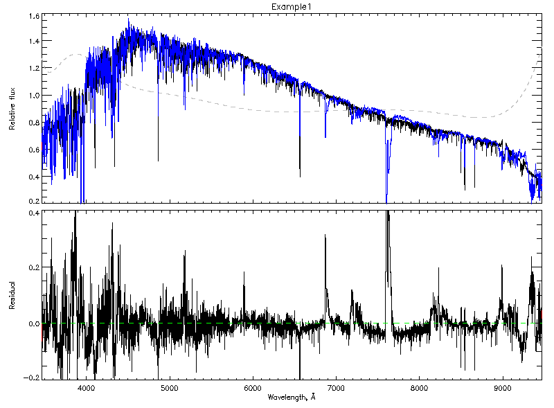
GDL> uly_solut_splot, solution, polycolor='Grey', polystyle=2, title='Example for plotting tutorial'
This way, anyone ignoring the existence of the plot_var structure will still be able to produce plots. Have a look at uly_plot_init for a full description of this structure and the plotting parameters. Alternatively, one can also use
GDL> help, uly_plot_init(), /STRUCTURE
** Structure <939338>, 32 tags, length=152, data length=140, refs=1:
   XSIZE           INT            700
   YSIZE           INT            500
   BGCOLOR         LONG               150
   AXISCOLOR       LONG               173
   HALFTONECT      INT             39
   LINECOLOR       LONG               183
   MODELCOLOR      STRING    'Blue'
   POLYCOLOR       STRING    'Cyan'
   RESIDCOLOR      STRING    'Black'
   SIGMACOLOR      STRING    'Green'
   BADCOLOR        STRING    'Red'
   PSYM            INT              0
   MODELPSYM       INT             10
   POLYPSYM        INT             10
   RESIDPSYM       INT             10
   SIGMAPSYM       INT              0
   LINESTYLE       INT              0
   MODELSTYLE      INT              0
   POLYSTYLE       INT              0
   RESIDSTYLE      INT              0
   SIGMASTYLE      INT              0
   LINETHICK       INT              1
   MODELTHICK      INT              1
   POLYTHICK       INT              1
   RESIDTHICK      INT              1
   SIGMATHICK      INT              1
   CHARSIZE        INT              1
   CHARTHICK       INT              1
   SHOWHALFTONE    INT              1
   SHOWCONTOUR     INT              1
   SHOWSIGMA       INT              0
   SHOWMINIMA      INT              1

to see what are to current values contained in the plot_var structure.

3. Advanced tip

If, after spending some time setting up plot_var to your liking, it is possible to save it using the buit-in IDL/GDL command save.
GDL> black_and_white = uly_plot_init()
GDL> black_and_white.linecolor=FSC_Color('Black')
GDL> black_and_white.modelcolor='Grey'
GDL> black_and_white.polycolor='Black'
GDL> black_and_white.polystyle=2
GDL> black_and_white.showsigma=0
GDL> 
GDL> uly_solut_splot, solution, PLOT_VAR=black_and_white
GDL> 
GDL> save, black_and_white, filename='bw_settings.sav'
These commands make the output plot to be in black and white. These black and white settings are then saved to a file called 'bw_settings.sav'. Later, you can use the command:
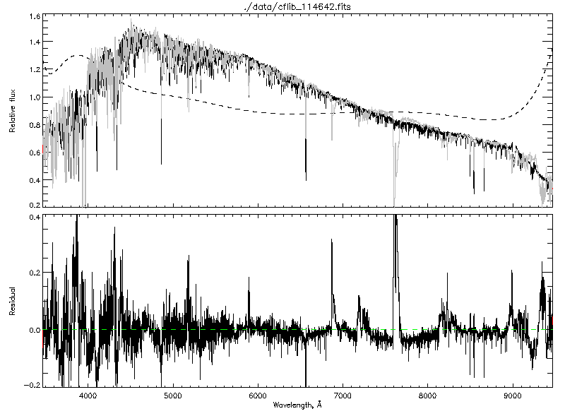
GDL> restore, 'bw_settings.sav'
this will restore the black_and_white structure and this can be reused.

4. Saving hardcopies

The task uly_plot_save allows to easily save jpg, png or tiff files.
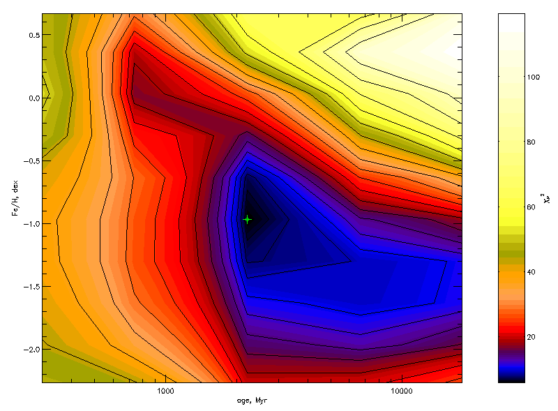
GDL> cmp = uly_ssp() 
GDL> chimap = uly_chimap(star, cmp, [[0,0],[0,1]], /QUIET)
GDL> plot_var = uly_plot_init(HALFTONECT=5)
GDL> uly_chimap_plot, chimap, /XLOG, XRANGE=[300., 18000.], PLOT_VAR=plot_var
GDL> uly_plot_save, 'filename.png', /PNG
will grab a screenshot of the plot and write it to filename.png. Note that the default behaviour for uly_plot_save is to write in PNG format and not in the popular JPG format. Because of its compression algorithm involving Fourier transforms, JPG is extremely bad at rendering scientific plots and all sharp lines become blury. The PNG format is therefore recomended for screenshots.
Contact: ulyss at obs.univ-lyon1.fr Last modified: Thu Jul 31 13:57:09 2008.