The application that drove the development of ULySS was the analyze
of stellar population. The goal was to fit in the same time
the internal kinematics and the characteristics (age, metallicity, ...)
of a galaxy.
In this tutorial we present examples of fit of stellar populations. First, SSP
and second composite populations.
GDL> cmp_peg = uly_ssp()
GDL> ulyss, uly_root+'/data/m67.fits', cmp_peg, FILE='m67_phr', /CLEAN, /QUIET
GDL> uly_solut_tprint, 'm67_phr'
cz             :       11.955643 +/- 0.43038056 km/s
dispersion     :       77.875987 +/- 0.44749150 km/s
-----------------------------------------------
estimated SNR  :      89.0879
-----------------------------------------------
cmp #0  cmp1
Weight         :   5.9871520e-13 +/-    7.5010847e-05 [data_unit/cmp_unit]
age            :       3766.7819 +/- 74.718439 Myr
Fe/H           :    -0.094549851 +/- 0.0059387329 dex
-----------------------------------------------
GDL> m67 = uly_root+'/data/m67.fits'
GDL> model = uly_ssp_extr(m67, uly_root+'/models/PHR_Elodie31.fits', [3920.,-0.1])
GDL> cmp = uly_star(model)
GDL> uly_lsf, m67, cmp, 400, 200, FILE='lsf_m67_phr.txt', /QUIET
GDL> uly_lsf_smooth, 'lsf_m67_phr.txt', 'lsfs_m67_phr.txt'
GDL> cmp_phr = uly_ssp(LSF='lsfs_m67_phr.txt')
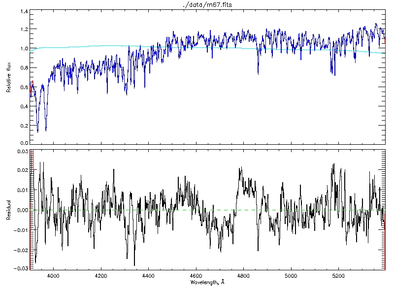
GDL> ulyss, m67, cmp_phr, KMOMENT=0, /CLEAN, FILE='m67_phr_2', /PLOT
Read the model ./models/PHR_Elodie31.fits
read the file ./models/PHR_Elodie31.fits
model reading time=       1.5694430
model deriving time=      0.12560892
--------------------------------------------------------------------
INPUT PARAMETERS
--------------------------------------------------------------------
The fits file to be analyze is       ./data/m67.fits
Name of the output file              m67_phr_2.res
Degree of multiplicative polynomial            10
No additive polynomial
Component1 (cmp2) model:./models/PHR_Elodie31.fits lsf:lsfs_m67_phr.txt
  Guess for age: 8000.0000 [Myr], Fe/H: -0.40000000 [dex]
--------------------------------------------------------------------
Read the model ./models/PHR_Elodie31.fits
read the file ./models/PHR_Elodie31.fits
model reading time=       1.5478568
model deriving time=      0.12618017
--------------------------------------------------------------------
PARAMETERS PASSED TO ULY_FIT
--------------------------------------------------------------------
Wavelength range used                 :       3900.4112       5397.5790
 [Angstrom]
Sampling in log wavelength            :       50.436632 [km/s]
Number of independent pixels in signal:        1931
Number of pixels fitted               :        1931
DOF factor                            :      1.00000
--------------------------------------------------------------------
number of model evaluations:          24
Number of clipped outliers:6+5+10 out of        1930  1.75902e-12
number of model evaluations:           8
time=      0.32360911
Number of pixels used for the fit        1910
-----------------------------------------------
estimated SNR  :       110.12712
-----------------------------------------------
cmp #0  cmp2
Weight         :   6.1476236e-13 +/-    7.7014466e-05 [data_unit/cmp_unit]
age            :       3866.2290 +/- 61.667604 Myr
Fe/H           :     -0.10462936 +/- 0.0041833108 dex
-----------------------------------------------
GDL> cmp_vaz = uly_ssp(MODEL=uly_root+'/models/Vaz_Miles.fits')
GDL> ulyss, uly_root+'/data/m67.fits', cmp_vaz, FILE='m67_vaz', /CLEAN, /QUIET, /PLO
GDL> uly_solut_tprint, 'm67_vaz'
cz             :       5.5566364 +/- 0.36412508 km/s
dispersion     :       45.649549 +/- 0.63828096 km/s
-----------------------------------------------
estimated SNR  :      89.3177
-----------------------------------------------
cmp #0  cmp1
Weight         :   3.8385023e-13 +/-    4.6707757e-05 [data_unit/cmp_unit]
age            :       3086.3486 +/- 30.706027 Myr
Fe/H           :    -0.027643403 +/- 0.0081537641 dex
-----------------------------------------------
GDL> m67 = uly_root+'/data/m67.fits'
GDL> model = uly_ssp_extr(m67, uly_root+'/models/Vaz_Miles.fits', [3920.,-0.1])
GDL> cmp = uly_star(model)
GDL> uly_lsf, m67, cmp, 400, 200, FILE='lsf_m67_vaz.txt', /QUIET
GDL> uly_lsf_smooth, 'lsf_m67_vaz.txt', 'lsfs_m67_vaz.txt'
GDL> cmp_vaz =  uly_ssp(MODEL=uly_root+'/models/Vaz_Miles.fits', LSF='lsfs_m67_vaz.txt')
GDL> ulyss, m67, cmp_vaz, KMOMENT=0, /CLEAN, FILE='m67_vaz_2', /PLOT
Read the model ./models/Vaz_Miles.fits
read the file ./models/Vaz_Miles.fits
model reading time=      0.49980402
model deriving time=     0.087624073
--------------------------------------------------------------------
INPUT PARAMETERS
--------------------------------------------------------------------
The fits file to be analyze is       ./data/m67.fits
Name of the output file              m67_vaz_2.res
Degree of multiplicative polynomial            10
No additive polynomial
Component1 (cmp2) model:./models/Vaz_Miles.fits lsf:lsfs_m67_vaz.txt
  Guess for age: 8000.0000 [Myr], Fe/H: -0.40000000 [dex]
--------------------------------------------------------------------
Read the model ./models/Vaz_Miles.fits
read the file ./models/Vaz_Miles.fits
model reading time=      0.48728895
model deriving time=     0.087376118
--------------------------------------------------------------------
PARAMETERS PASSED TO ULY_FIT
--------------------------------------------------------------------
Wavelength range used                 :       3634.9308       5397.5790
 [Angstrom]
Sampling in log wavelength            :       50.436632 [km/s]
Number of independent pixels in signal:        2350
Number of pixels fitted               :        2350
DOF factor                            :      1.00000
--------------------------------------------------------------------
number of model evaluations:          23
Number of clipped outliers:1+0+0 out of        2347  1.33916e-12
number of model evaluations:          41
time=      0.54413891
Number of pixels used for the fit        2346
-----------------------------------------------
estimated SNR  :       124.89012
-----------------------------------------------
cmp #0  cmp2
Weight         :   3.7134409e-13 +/-    4.5184716e-05 [data_unit/cmp_unit]
age            :       2893.2265 +/- 19.765443 Myr
Fe/H           :     0.024110728 +/- 0.0061693286 dex
-----------------------------------------------
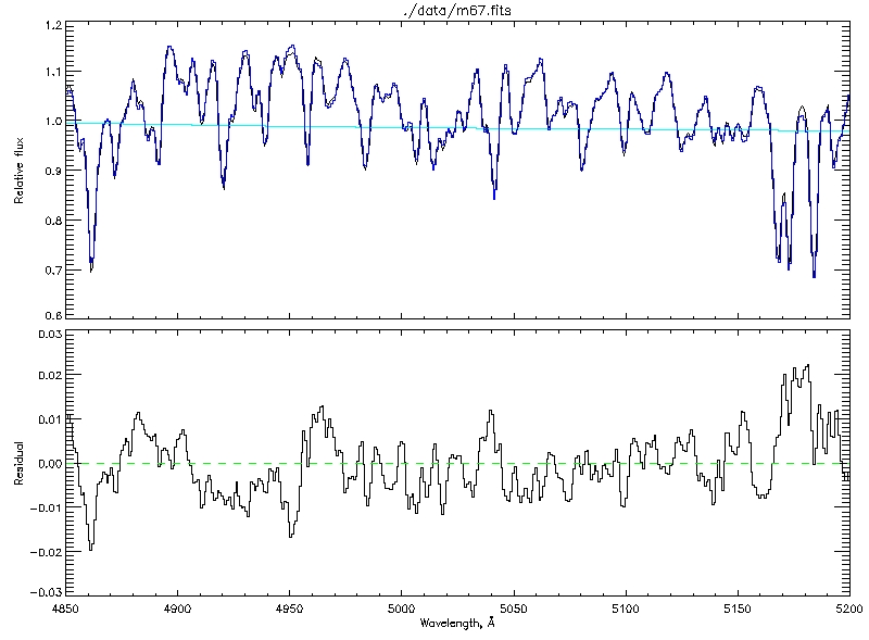
GDL> window, 0
GDL> uly_solut_splot, 'm67_phr_2', WAVERANGE=[4850.,5200.], RESI_YR=[-0.03, 0.03]
GDL> window, 1
GDL> uly_solut_splot, 'm67_vaz_2', WAVERANGE=[4850.,5200.], RESI_YR=[-0.03, 0.03]
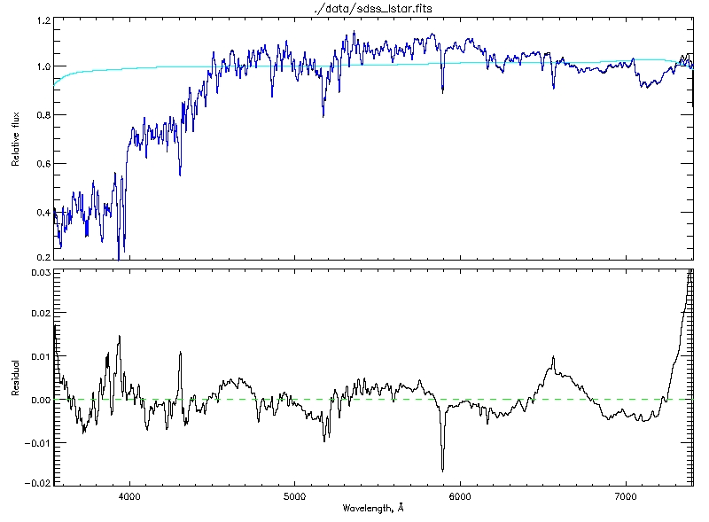
GDL> ulyss, uly_root+'/data/sdss_lstar.fits', MODEL=uly_root+'/models/Vaz_Miles.fits', /PLOT
--------------------------------------------------------------------
INPUT PARAMETERS
--------------------------------------------------------------------
The fits file to be analyze is       ./data/sdss_lstar.fits
Name of the output file              output.res
Degree of multiplicative polynomial            10
No additive polynomial
Component1 (cmp1) model:./models/Vaz_Miles.fits
  Guess for age: 8000.0000 [Myr], Fe/H: -0.40000000 [dex]
--------------------------------------------------------------------
Convert axis scale from log10 to log
Read the model ./models/Vaz_Miles.fits
read the file ./models/Vaz_Miles.fits
model reading time=      0.71985984
model deriving time=      0.17039514
--------------------------------------------------------------------
PARAMETERS PASSED TO ULY_FIT
--------------------------------------------------------------------
Wavelength range used                 :       3540.5000       7410.3298
 [Angstrom]
Sampling in log wavelength            :       51.507049 [km/s]
Number of independent pixels in signal:        4299
Number of pixels fitted               :        4299
DOF factor                            :      1.00000
--------------------------------------------------------------------
number of model evaluations:          44
time=      0.75634599
Number of pixels used for the fit        4298

cz             :      -1.4282577 +/- 1.3877349 km/s
dispersion     :       250.53003 +/- 1.3348753 km/s
-----------------------------------------------
estimated SNR  :       90.982289
-----------------------------------------------
cmp #0  cmp1
Weight         :   2.2649453e-10 +/-    4.3723515e-05 [data_unit/cmp_unit]
age            :       4504.0522 +/- 157.40854 Myr
Fe/H           :   -0.0067877102 +/- 0.0056177991 dex
-----------------------------------------------
GDL> ulyss, uly_root+'/data/sdss_star.fits', model=uly_root+'/models/elodie32_flux_tgm.fits', MD=70
--------------------------------------------------------------------
INPUT PARAMETERS
--------------------------------------------------------------------
The fits file to be analyze is       ./data/sdss_star.fits
Name of the output file              output.res
Degree of multiplicative polynomial        70
No additive polynomial
Component1 (cmp1) model:./models/elodie32_flux_tgm.fits
  Guess for Teff: 7000.0000 [K], Logg: 2.0000000 [cm/s2], Fe/H: 0.0000000 [dex]
--------------------------------------------------------------------
--------------------------------------------------------------------
PARAMETERS PASSED TO ULY_FIT
--------------------------------------------------------------------
Wavelength range used                 :       3900.5998       6800.3525
 [Angstrom]
Sampling in log wavelength            :       69.029774 [km/s]
Number of independent pixels in signal:        2414
Number of pixels fitted               :        2414
DOF factor                            :      1.00000
--------------------------------------------------------------------
number of model evaluations:          38
time=       2.4529600
Number of pixels used for the fit        2389

cz             :       125.49753 +/- 0.00023862830 km/s
dispersion     :       70.811303 +/- 0.00024744205 km/s
-----------------------------------------------
chi^2          :       7106302.8
-----------------------------------------------
cmp #0  cmp1
Weight         :       13180.012 +/-     0.0018750643 [data_unit/cmp_unit]
Teff           :       4765.9682 +/- 0.0067990484 K
Logg           :       2.9178982 +/- 1.5327789e-05 cm/s2
Fe/H           :    -0.010886753 +/- 6.7127836e-06 dex
-----------------------------------------------
GDL> star = uly_root+'/data/sdss_star.fits'
GDL> model = uly_tgm_extr(star,[4700.,3.,0.])
GDL> cmp = uly_tgm(TG=4700, LG=3., ZG=0)
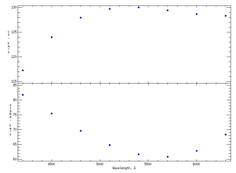
GDL> uly_lsf, star, cmp, 600, 300, FIL='sdss_lsf.txt', /QUIET
GDL> uly_lsf_smooth, 'sdss_lsf.txt', 'sdss_lsfs.txt'
GDL> uly_lsf_plot, 'sdss_lsfs.txt'
GDL> cmp = uly_ssp(MODEL='PHR_Elodie31_SDSS.fits')
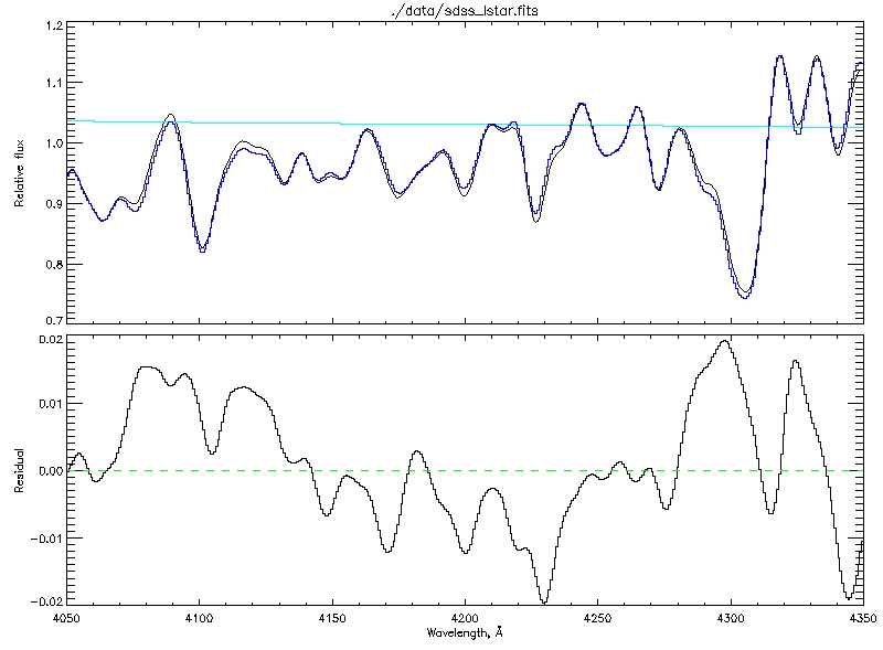
GDL> ulyss, uly_root+'/data/sdss_lstar.fits', cmp, FILE='sdss', /QUIET
GDL> window, 0
GDL> uly_solut_splot, 'sdss', WAVERANGE=[4050, 4350]
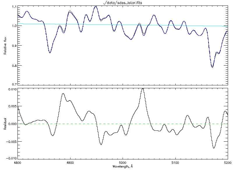
GDL> window, 1
GDL> uly_solut_splot, 'sdss', WAVERANGE=[4800, 5200]
GDL> cmp1 = uly_ssp(MODEL='PHR_Elodie31_SDSS.fits', AG=[500.])
GDL> cmp2 = uly_ssp(MODEL='PHR_Elodie31_SDSS.fits', AG=[2000.])
GDL> cmp3 = uly_ssp(MODEL='PHR_Elodie31_SDSS.fits', AG=[12000.])
GDL> cmp = [cmp1, cmp2, cmp3]
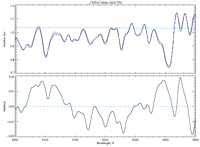
GDL> ulyss, uly_root+'/data/sdss_lstar.fits', cmp, FILE='sdss'
GDL> window, 0
GDL> uly_solut_splot, 'sdss', WAVERANGE=[4050, 4350]
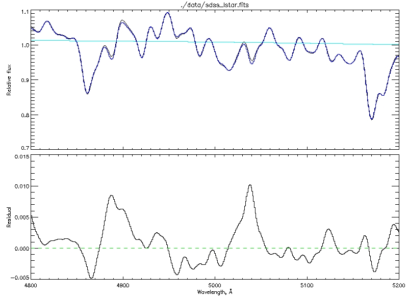
GDL> window, 1
GDL> uly_solut_splot, 'sdss', WAVERANGE=[4800, 5200]
--------------------------------------------------------------------
INPUT PARAMETERS
--------------------------------------------------------------------
The fits file to be analyze is       ./data/sdss_lstar.fits
Name of the output file              sdss.res
Degree of multiplicative polynomial            10
No additive polynomial
Component1 (cmp1) model:PHR_Elodie31_SDSS.fits
  Guess for age: 500.00000 [Myr], Fe/H: -0.40000000 [dex]
Component2 (cmp2) model:PHR_Elodie31_SDSS.fits
  Guess for age: 2000.0000 [Myr], Fe/H: -0.40000000 [dex]
Component3 (cmp3) model:PHR_Elodie31_SDSS.fits
  Guess for age: 12000.000 [Myr], Fe/H: -0.40000000 [dex]
--------------------------------------------------------------------
Convert axis scale from log10 to log
Read the model PHR_Elodie31_SDSS.fits
read the file PHR_Elodie31_SDSS.fits
model reading time=       1.7748680
model deriving time=      0.21680212
Read the model PHR_Elodie31_SDSS.fits
read the file PHR_Elodie31_SDSS.fits
model reading time=       1.7646132
model deriving time=      0.21615505
Read the model PHR_Elodie31_SDSS.fits
read the file PHR_Elodie31_SDSS.fits
model reading time=       1.7665751
model deriving time=      0.21738100
--------------------------------------------------------------------
PARAMETERS PASSED TO ULY_FIT
--------------------------------------------------------------------
Wavelength range used                 :       3900.7477       6800.3252
 [Angstrom]
Sampling in log wavelength            :       51.507049 [km/s]
Number of independent pixels in signal:        3235
Number of pixels fitted               :        3235
DOF factor                            :      1.00000
--------------------------------------------------------------------
number of model evaluations:         194
time=       2.3005202
Number of pixels used for the fit        3172

cz             :      0.13893332 +/- 0.88427811 km/s
dispersion     :       256.33691 +/- 0.86741092 km/s
-----------------------------------------------
estimated SNR  :       172.38968
-----------------------------------------------
cmp #0  cmp1
Light fraction :       3.5823853 +/-        54405689. %
Weight         :   1.8041577e-12 +/-    2.7399745e-05 [data_unit/cmp_unit]
age            :       1437.6185 +/- 294.95920 Myr
Fe/H           :      -2.3010299 dex (pegged at low bound)
-----------------------------------------------
cmp #2  cmp3
Light fraction :       96.417615 +/-        55921113. %
Weight         :   3.5946363e-10 +/-    0.00020848479 [data_unit/cmp_unit]
age            :       5316.5201 +/- 90.044115 Myr
Fe/H           :     0.017911459 +/- 0.0040683910 dex
-----------------------------------------------
The following component(s) had no contribution
1(cmp2)
-----------------------------------------------